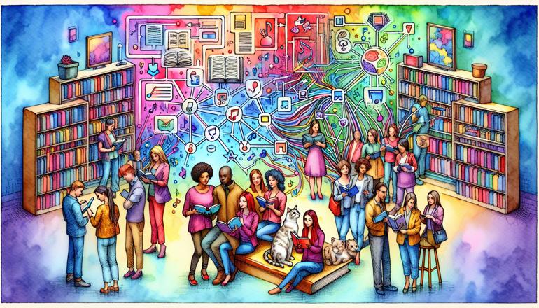
Collaborative Filtering Explained
Imagine you're trying to pick a new movie to watch, but there are too many options. You ask your friends what they liked, especially those whose tastes align with yours. If they loved a film, chances are you might enjoy it too. That's the essence of collaborative filtering – it's a technique used in recommendation systems to predict what you might like based on the preferences of similar users or similar items.
In the digital world, collaborative filtering is the backbone of many platforms you use daily. When Netflix suggests a show, Amazon recommends a product, or Spotify creates a personalized playlist, they're likely using some form of collaborative filtering. It works by collecting preferences from many users and using that data to generate recommendations for individuals.
There are two main approaches to collaborative filtering: user-based and item-based. User-based collaborative filtering finds users similar to you and recommends items those similar users have liked. Item-based collaborative filtering looks at items similar to those you've already enjoyed and suggests those similar items.
Let's look at a simple example. Suppose we have a small dataset of user ratings for movies:
| User | Movie A | Movie B | Movie C | Movie D |
|---|---|---|---|---|
| Alice | 5 | 3 | 4 | ? |
| Bob | 4 | ? | 3 | 5 |
| Carol | ? | 4 | 5 | 2 |
| Dave | 2 | 5 | ? | 4 |
In this table, question marks represent missing ratings that we want to predict. For example, we might want to predict what rating Alice would give to Movie D.
To implement collaborative filtering in Python, we typically use libraries like Surprise or Scikit-learn. Here's a basic example using cosine similarity for user-based collaborative filtering:
import numpy as np
from sklearn.metrics.pairwise import cosine_similarity

# User-item matrix (rows: users, columns: movies)
ratings = np.array([
    [5, 3, 4, 0],  # Alice (0 for missing rating)
    [4, 0, 3, 5],  # Bob
    [0, 4, 5, 2],  # Carol
    [2, 5, 0, 4]   # Dave
])

# Calculate user similarities
user_similarities = cosine_similarity(ratings)

# Predict missing ratings
def predict_rating(user_idx, item_idx):
    numerator = 0
    denominator = 0
    for other_user in range(len(ratings)):
        if other_user != user_idx and ratings[other_user][item_idx] != 0:
            similarity = user_similarities[user_idx][other_user]
            numerator += similarity * ratings[other_user][item_idx]
            denominator += abs(similarity)
    return numerator / denominator if denominator != 0 else 0

# Predict Alice's rating for Movie D
predicted_rating = predict_rating(0, 3)
print(f"Predicted rating for Alice on Movie D: {predicted_rating:.2f}")
This code calculates how similar users are to each other using cosine similarity, then uses those similarities to weight the ratings from similar users when making predictions.
User-based collaborative filtering works particularly well when you have a dense dataset with many ratings per user. The key steps involve: - Calculating similarity between users - Selecting the most similar users (neighbors) - Combining their ratings to make predictions
The similarity between users can be measured using various metrics. The most common ones include:
- Pearson correlation coefficient
- Cosine similarity
- Euclidean distance
- Jaccard similarity
Each metric has its strengths and weaknesses depending on your data characteristics. Pearson correlation handles differences in rating scales well, while cosine similarity works better with sparse data.
Now let's look at the other approach. Item-based collaborative filtering focuses on the relationships between items rather than users. It works by finding items that are similar to those a user has already rated highly, then recommending those similar items.
Here's a simple implementation of item-based collaborative filtering:
# Calculate item similarities
item_similarities = cosine_similarity(ratings.T)  # Transpose for item-based

def predict_rating_item_based(user_idx, item_idx):
    numerator = 0
    denominator = 0
    user_ratings = ratings[user_idx]
    for other_item in range(len(user_ratings)):
        if other_item != item_idx and user_ratings[other_item] != 0:
            similarity = item_similarities[item_idx][other_item]
            numerator += similarity * user_ratings[other_item]
            denominator += abs(similarity)
    return numerator / denominator if denominator != 0 else 0

# Predict Alice's rating for Movie D using item-based approach
predicted_rating_item = predict_rating_item_based(0, 3)
print(f"Item-based predicted rating: {predicted_rating_item:.2f}")
Item-based filtering often performs better in practice because item relationships tend to be more stable than user relationships. People's tastes might change over time, but if two movies are similar, they'll likely remain similar.
Both approaches face common challenges in real-world applications. The cold start problem occurs when new users or items have little to no rating data, making it difficult to generate accurate recommendations. Data sparsity is another issue - most users rate only a small fraction of available items, creating a sparse matrix that's challenging to work with.
Here's a comparison of the two main approaches:
| Aspect | User-Based | Item-Based |
|---|---|---|
| Performance | Slower with many users | Faster, more scalable |
| Stability | User preferences change | Item relationships stable |
| Cold Start | Hard for new users | Hard for new items |
| Interpretation | "Users like you also liked..." | "Because you liked X, you might like Y" |
Modern recommendation systems often use matrix factorization techniques, which are more advanced forms of collaborative filtering. These methods factorize the user-item matrix into lower-dimensional matrices that capture latent features of both users and items.
from sklearn.decomposition import NMF

# Using Non-negative Matrix Factorization
model = NMF(n_components=2, init='random', random_state=42)
W = model.fit_transform(ratings)  # User features
H = model.components_             # Item features

# Reconstruct the matrix to get predictions
predictions = np.dot(W, H)
print("NMF predictions:")
print(predictions)
Matrix factorization techniques like Singular Value Decomposition (SVD) and Non-negative Matrix Factorization (NMF) can handle sparse data better and often provide more accurate recommendations than neighborhood-based methods.
When implementing collaborative filtering, there are several important considerations to keep in mind. You need to choose appropriate similarity metrics, handle missing data properly, and consider computational efficiency. For large-scale systems, you might need distributed computing frameworks like Apache Spark.
Evaluation is crucial for any recommendation system. Common evaluation metrics include:
- Mean Absolute Error (MAE)
- Root Mean Square Error (RMSE)
- Precision and Recall
- Normalized Discounted Cumulative Gain (NDCG)
These metrics help you understand how well your system is performing and guide improvements.
Real-world applications of collaborative filtering extend beyond entertainment recommendations. They're used in e-commerce for product recommendations, in news platforms for article suggestions, in dating apps for match recommendations, and even in educational systems for suggesting learning materials.
One significant challenge is avoiding the filter bubble effect, where users only see content similar to what they already like, potentially limiting their exposure to diverse content. Many platforms now incorporate diversity measures to ensure recommendations include some serendipitous discoveries.
Another consideration is privacy. Collaborative filtering requires collecting user data, which raises privacy concerns. Techniques like differential privacy and federated learning are emerging to address these concerns while still enabling effective recommendations.
The field continues to evolve with new techniques emerging regularly. Deep learning approaches using neural networks have shown promising results, often outperforming traditional collaborative filtering methods. These models can capture complex nonlinear relationships in the data.
Here's a simple example using a neural network for collaborative filtering:
from tensorflow.keras.models import Model
from tensorflow.keras.layers import Input, Embedding, Flatten, Dot

# Number of users and items
n_users = 4
n_items = 4
embedding_size = 10

# User embedding
user_input = Input(shape=[1])
user_embedding = Embedding(n_users, embedding_size)(user_input)
user_vec = Flatten()(user_embedding)

# Item embedding
item_input = Input(shape=[1])
item_embedding = Embedding(n_items, embedding_size)(item_input)
item_vec = Flatten()(item_embedding)

# Dot product of user and item embeddings
prod = Dot(axes=1)([user_vec, item_vec])

model = Model([user_input, item_input], prod)
model.compile('adam', 'mean_squared_error')
This neural network approach learns embeddings for users and items that capture their latent features, then uses the dot product of these embeddings to predict ratings.
Despite the advances in deep learning, traditional collaborative filtering methods remain relevant because they're often easier to implement, interpret, and require less computational resources. Many production systems use hybrid approaches that combine multiple techniques.
When building your own recommendation system, start with simple collaborative filtering methods and gradually incorporate more advanced techniques as needed. Always focus on understanding your data and the specific requirements of your application rather than blindly applying the latest algorithm.
Remember that no single approach works best for all scenarios. The effectiveness of collaborative filtering depends on your specific data characteristics, business requirements, and user behavior patterns. Experimentation and continuous evaluation are key to building successful recommendation systems.
Collaborative filtering has revolutionized how we discover content and products online. By understanding how these systems work, you can build better recommendations for your users while being mindful of the ethical considerations involved. Whether you're building a small website or a large-scale platform, collaborative filtering provides powerful tools for creating personalized experiences.


